Using PyTorch to identify respiratory problems through chest X-rays

Introduction

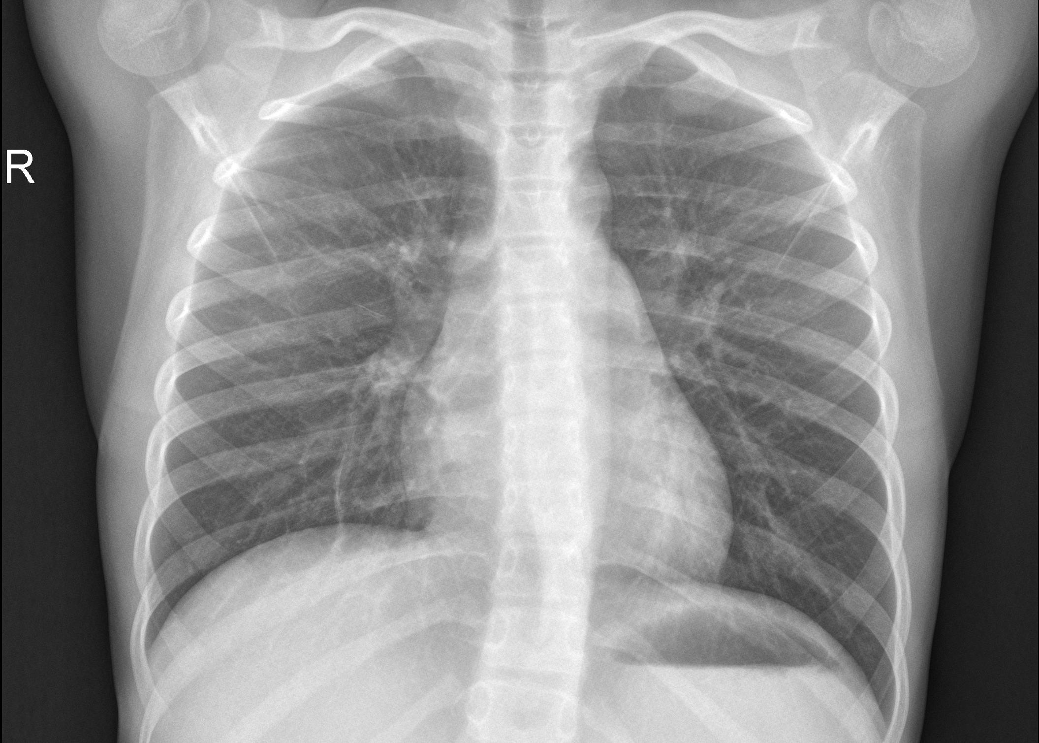
I have recently become interested in machine learning (ML) and the seemingly endless list of tasks which it can help with. Because of this, I have spent a good amount of time in the last few months learning it through tutorials, documentation, and side projects. When looking for some inspiration for what to make with PyTorch, I came across this Kaggle repository which had over 7,000 photos of chest x-rays from people with COVID-19, Tuberculosis, Pneumonia, or just a normal chest. This specifically caught my attention as it would be building a tool to accomplish a task that I am fully unable to do due to lacking the necessary background.

Process

Starting off, turning the data into tensors is a vital part of making an algorithm, but to make it more visual, I like to put an image of the data on coordinates to help visualize the number of pixels, and thus data within it.

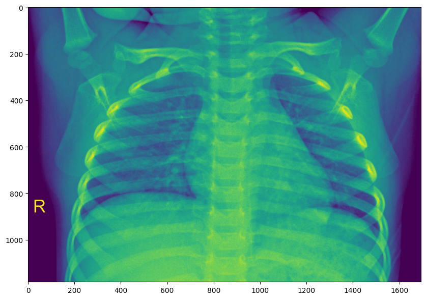
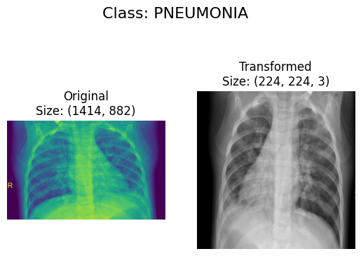
Then, to ensure all pictures are the same size, and carry the same amount of data, all images must be transformed to the same size. Additionally, it is important to apply some transformations to create some diversity in the data. Then, the data needs to be turned into tensors which allows the model to understand the data. Below is how I made the transformations for the data.

data_transform = transforms.Compose([
    transforms.Resize(size=(224,224)), #changes the number of pixels  in the image to 224 x 224
    transforms.Lambda(lambda img: img.convert("RGB")), #makes sure all images have 3 colour channels
    transforms.RandomHorizontalFlip(p=0.5), #creates diversity in the data by flipping half of the images
    transforms.TrivialAugmentWide(num_magnitude_bins=31), # Further makes diversity by applying a series of random transformations
    transforms.ToTensor() #transforms the images into tensors
])

And this resulted in the following:

To prepare this data efficiently for the model, a data loader is needed. This is done fairly simply as PyTorch streamlines the process

# Create DataLoaders
BATCH_SIZE = 32
NUM_WORKERS = os.cpu_count()
train_dataloader_simple = DataLoader(train_data_simple,
                                     batch_size=BATCH_SIZE,
                                     shuffle=True,
                                     num_workers=NUM_WORKERS)

For the small convolutional neural network, it processes images through two blocks to extract the features, then flattens and passes it through a linear layer to give output predictions

def __init__(self, input_shape: int, hidden_units: int, output_shape: int, image_size: int) -> None:
        super().__init__()
        self.conv_block_1 = nn.Sequential( #First sequential layer assigned 
            nn.Conv2d(in_channels=input_shape, out_channels=hidden_units, kernel_size=3, stride=1, padding=1), # First convolutional layer
            nn.ReLU(), # (Rectified Linear Unit), adds non-linearity by zeroing out negative values
            nn.Conv2d(in_channels=hidden_units, out_channels=hidden_units, kernel_size=3, stride=1, padding=1),
            nn.ReLU(),
            nn.MaxPool2d(kernel_size=2, stride=2) # reduce spatial dimensions by half and moves 2 pixels  at a time
            #this basically summarizes the images for the model
        )
        self.conv_block_2 = nn.Sequential(
            nn.Conv2d(hidden_units, hidden_units, kernel_size=3, padding=1),
            nn.ReLU(),
            nn.Conv2d(hidden_units, hidden_units, kernel_size=3, padding=1),
            nn.ReLU(),
            nn.MaxPool2d(2)
        )

        with torch.no_grad():
            dummy_input = torch.zeros(1, input_shape, image_size, image_size) # makes tensor full of 0's
            out = self.conv_block_1(dummy_input) #passes on the dummy input
            out = self.conv_block_2(out) #Passes the output from the first block through the second convolutional block 
            flatten_dim = out.view(1, -1).shape[1] #dynamically calculate how many input features should be expected

        self.classifier = nn.Sequential(
            nn.Flatten(),
            nn.Linear(in_features=flatten_dim, out_features=output_shape)
        )

    def forward(self, x: torch.Tensor):
        x = self.conv_block_1(x)
        x = self.conv_block_2(x)
        x = self.classifier(x)
        return x #passes the value through the conv layers and returns the output

After this, the model must step forward and repeat to continue working properly. This requires the loss to be accumulated, an optimizer applied (zero_grad in this case), backpropagation, and an optimizer step where the bias and weight are updated.

Training and results

By setting a number of Epochs, the model can be trained and worked through that many times. This model took about ten minutes to train on Google Colab T4 GPUs and resulted in an accuracy of 81.25%. Below, a few examples of results and confidence are shown.

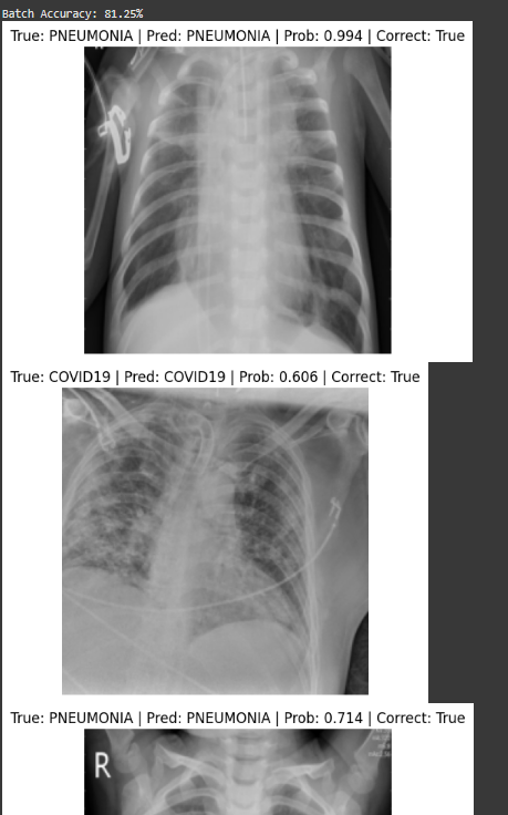
To see why the results had some error, I graphed the loss and accuracy and found a slight tendency to overfit, which may be caused by the lack of variation in the data, which could be adjusted in the future. Despite this, the overall trend seems to be going in the right direction.

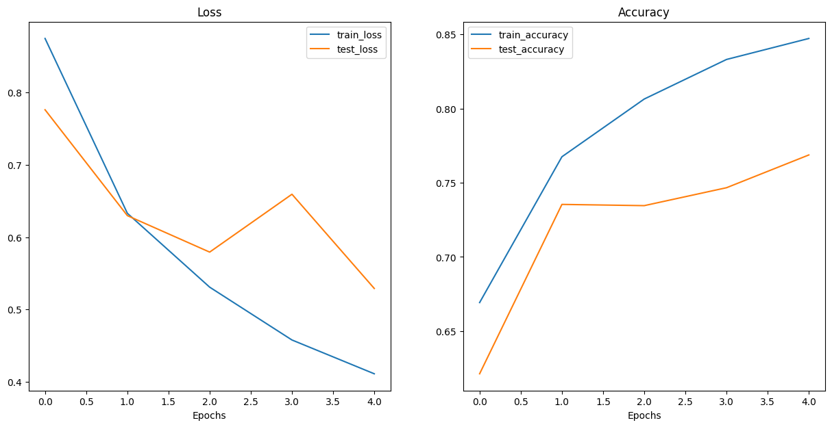
Going forward, the optimizer method should be experimented with to see if the overall accuracy can be improved. On top of this, larger picture sizes would allow a greater level of detail to be maintained which could also serve to increase the accuracy. However, the great thing about ML is how it encourages experimentation and trial and error, as that is often the best way forward when there is no specific path.